MLPs Classification of the MNIST Dataset

This notebook demonstrates how to use a Multi-Layer Perceptron (MLPs) neural network to classify handwritten digits from the MNIST dataset. MLPs use fully-connected hidden layers in their stucture.

The MNIST dataset contains 70,000 grayscale images of handwritten digits (0-9), each with a size of 28x28 pixels.

Dataset split: - Training set: 60,000 images - Test set: 10,000 images

Target variable: Digit class (0-9)

Import Modules

import numpy as np
import matplotlib.pyplot as plt
import tensorflow as tf
from tensorflow import keras
from tensorflow.keras.models import Model
from tensorflow.keras.layers import Input, Dense, Flatten
from sklearn.metrics import accuracy_score, classification_report, confusion_matrix

Load the MNIST Dataset

# Load the dataset from keras datasets
(X_train, y_train), (X_test, y_test) = keras.datasets.mnist.load_data()

# Display the shape of training and test data
print(X_train.shape)
print(X_test.shape)
# Each image has 28x28 pixels

(60000, 28, 28)
(10000, 28, 28)

# Display 9 images from the training set adn their labels
plt.figure(figsize=(9, 6))
for n in range(9):
    i = np.random.randint(0, len(X_train), 1)
    ax = plt.subplot(3, 3, n+1)
    plt.imshow(X_train[i[0]], cmap='gray')
    plt.title('Label:' + str(y_train[i[0]]))
    plt.axis('off')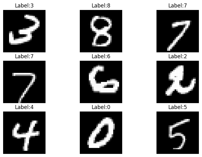

Data Preprocessing

# Normalize pixel values to range [0, 1]
X_train = X_train.astype('float32') / 255.0
X_test = X_test.astype('float32') / 255.0

# Flatten the images from 28x28 to 784-dimensional vectors
X_train = X_train.reshape(-1, 28 * 28)
X_test = X_test.reshape(-1, 28 * 28)

# Print the shapes of data and label sets
print('Training data features', X_train.shape)
print('Training labels', y_train.shape)
print('Testing data features', X_test.shape)
print('Testing labels', y_test.shape)

Training data features (60000, 784)
Training labels (60000,)
Testing data features (10000, 784)
Testing labels (10000,)

Build the MLP Model

# Define the layers in the MLP neural network
# Input layer - 784 features
inputs = Input(shape=(784,))
dense1 = Dense(units=512, activation='relu')(inputs)
dense2 = Dense(units=256, activation='relu')(dense1)
# Output layer - 10 classes
outputs = Dense(units=10, activation='softmax')(dense2)

# Define the model by providing the inputs and outputs
model = Model(inputs, outputs)

Train the MLP Model

# Compile the model
model.compile(optimizer='adam', loss='sparse_categorical_crossentropy', metrics=['accuracy'])

# Fit the model to the training dataset
history = model.fit(X_train, y_train, epochs=5, validation_split=0.2, verbose=1)

Epoch 1/5

1500/1500 ━━━━━━━━━━━━━━━━━━━━ 20s 12ms/step - accuracy: 0.8937 - loss: 0.3521 - val_accuracy: 0.9658 - val_loss: 0.1145

Epoch 2/5

1500/1500 ━━━━━━━━━━━━━━━━━━━━ 21s 14ms/step - accuracy: 0.9738 - loss: 0.0858 - val_accuracy: 0.9696 - val_loss: 0.1024

Epoch 3/5

1500/1500 ━━━━━━━━━━━━━━━━━━━━ 18s 12ms/step - accuracy: 0.9814 - loss: 0.0566 - val_accuracy: 0.9746 - val_loss: 0.0933

Epoch 4/5

1500/1500 ━━━━━━━━━━━━━━━━━━━━ 17s 12ms/step - accuracy: 0.9863 - loss: 0.0417 - val_accuracy: 0.9737 - val_loss: 0.1004

Epoch 5/5

1500/1500 ━━━━━━━━━━━━━━━━━━━━ 17s 12ms/step - accuracy: 0.9904 - loss: 0.0283 - val_accuracy: 0.9727 - val_loss: 0.1084

# Plot the accuracy and loss
train_loss = history.history['loss']
val_loss = history.history['val_loss']
acc = history.history['accuracy']
val_acc = history.history['val_accuracy']

epochsn = np.arange(1, len(train_loss)+1,1)
plt.figure(figsize=(12, 4))

plt.subplot(1,2,1)
plt.plot(epochsn, acc, 'b', label='Training Accuracy')
plt.plot(epochsn, val_acc, 'r', label='Validation Accuracy')
plt.grid(color='gray', linestyle='--')
plt.legend()
plt.title('ACCURACY')
plt.xlabel('Epochs')
plt.ylabel('Accuracy')

plt.subplot(1,2,2)
plt.plot(epochsn,train_loss, 'b', label='Training Loss')
plt.plot(epochsn,val_loss, 'r', label='Validation Loss')
plt.grid(color='gray', linestyle='--')
plt.legend()
plt.title('LOSS')
plt.xlabel('Epochs')
plt.ylabel('Loss')
plt.show()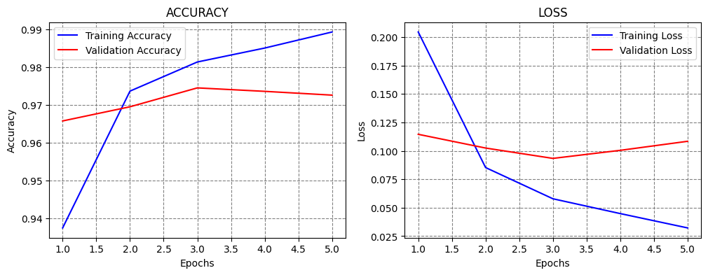

Evaluate the Model

# Calculate and print the accuracy on the test dataset
evals_test = model.evaluate(X_test, y_test)
print(f"Accuracy on test dataset: {evals_test[1]*100:5.2f}%")

313/313 ━━━━━━━━━━━━━━━━━━━━ 2s 6ms/step - accuracy: 0.9732 - loss: 0.1119

Accuracy on test dataset: 97.57%

# Predict on test dataset
y_pred_probabilities = model.predict(X_test)
model_predictions = np.argmax(y_pred_probabilities, axis=1)

313/313 ━━━━━━━━━━━━━━━━━━━━ 1s 3ms/step

# Print confusion matrix
print("Confusion Matrix:")
print(confusion_matrix(y_test, model_predictions))

Confusion Matrix:
[[ 972    1    1    0    1    0    1    1    1    2]
 [   0 1130    2    1    0    0    0    0    2    0]
 [   2    1 1014    2    2    0    1    8    2    0]
 [   0    0    7  992    0    2    0    4    5    0]
 [   1    4    3    2  959    0    3    3    0    7]
 [   3    0    0   36    0  841    3    2    5    2]
 [   4    3    3    0    5    3  934    1    5    0]
 [   0   10    8    5    0    0    0 1003    0    2]
 [   3    2    5   12    4    2    0   10  930    6]
 [   3    2    0    7    7    2    0    6    0  982]]

The confusion matrix shows the classification results for each digit (0-9): - Diagonal elements: Correctly classified digits - Off-diagonal elements: Misclassifications (showing which digits were confused with each other)